|
|
|
|
|
|
| Home | Company Info | Blog | Tutorials & Tools | Forums | Store | Services | Contact | Site Map |
HFSS Tutorial 3 |
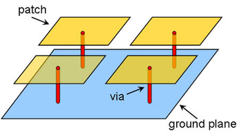
Dispersion Diagram II: Sievenpiper MushroomHFSSv10 (download simulation file) The Sievenpiper mushroom structure has been widely studied in the microwave engineering field due to its unique properties. The Sievenpiper mushroom structure basically consists of a metallic patch connected to ground with a shorting post. The general model is shown in Fig. 1.
It can be used as a high-impedance surface and act like a artifical magnetic conductor. The Sievenpiper mushroom structure has also been widely used to realize left-handed metamaterials (negative refractive index) since it can be designed to support a dominant quasi-TEM backward wave (i.e. anti-parallel group and phase velocities). In this tutorial, the dispersion diagram of a left-handed Sievenpiper mushroom structure is generated using HFSS's eigenmode solver. For a review on dispersion diagrams please refer to Tutorial I. The following topics are covered:
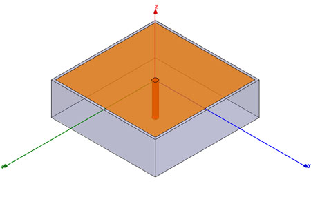
Model SetupFirst we must configure HFSS to use its eigenmode solver; HFSS>Solution Type...>Eigenmode. Next, the unit-cell of the Sievenpiper mushroom structure has to be drawn in HFSS. It consists of a square patch, a via, and a square block of substrate as shown in Fig. 2. The dimensions of the patch is 4.8x4.8 mm2 and is assigned a PEC boundary condition. The via has a radius of 0.12 mm, a height of 1.27 mm, and is assigned a perfect conductor material. In the case of the substrate, its dimensions are 5.0x5.0x1.27 mm3 and the substrate material is Rogers RT/duroid 6010/6010LM.
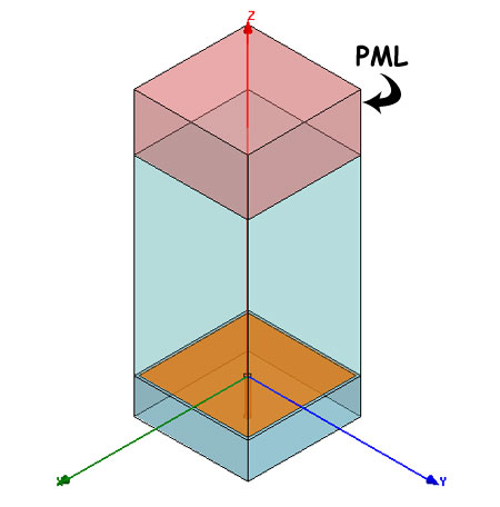
Since the Sievenpiper structure is open to air in the positive z-direction, an airbox has to be defined for the simulation. To simulate an infinite free space, a perfect matched layer (PML) boundary is defined on top of the airbox as shown in Fig. 3. Radiation boundary cannot be used in the eigenmode simulation. The height of the airbox has to be approximately six times the substrate thickness. The default values for the PML boundary condition are used.
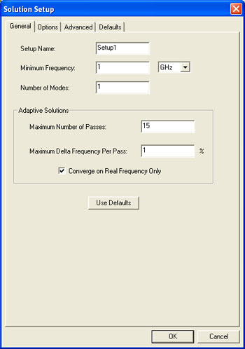
Periodic Boundary ConditionsPeriodic boundary conditions must be applied to the face of the entire structure, which includes the airbox and the PML. Therefore, another airbox has to be created with encloses the original airbox and PML. Master and slave boundaries are then applied just as in Tutorial I. The only difference is that I separated the simulation into three designs, one for each part of the Brillouin zone and only px is defined and is used for sweeping. You can use the same setup as the parallel plate simulation. Analysis/Optometrics SetupBefore the eigenmode analysis can be started, several steps need to be completed first. First, add a solution setup and input the values as depicted in Fig. 4. In addition, in the options tab of the Solutions Setup, input a minimum converged passes of 2. Note that the mesh gets large (around 30,000 tets) for each eigenpoint. As a result, this simulation takes several hours even for only one mode.
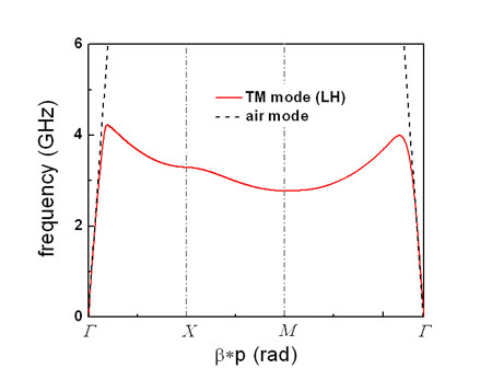
Next, parametric sweeps are added for each design in the simulation file. For the first parametric sweep, we will go from Г to Х and this design is labeled 1_Gamma2X. Add a linear step sweep for the variable px from 15 deg to 180 deg with 15 deg steps. In the Options tab make sure to check both Save Fields and Mesh and Copy geometrically equivalent meshes. For the second parametric sweep, we will go from Х to M and this design is will be labeled 2_X2M. For the sx boundary, the phase delay is set to 180, while the sy boundary has a phase delay of px. Add a linear step sweep for the variable px from 15 deg to 180 deg with 15 deg steps. In the options tab make sure to check both Save Fields and Mesh and Copy geometrically equivalent meshes. For the third parametric sweep, we will go from M to Г and this design will be labeled 3_M2Gamma. For this case, both the sx and sy boundaries are set to have a phase delay of px. Add a linear step sweep for the variable px from 15 deg to 180 deg with 15 deg steps. In the options tab make sure to check both Save Fields and Mesh and Copy geometrically equivalent meshes. Plotting ResultsSince each part of the Brillouin zone is done in a separate design, plotting the results is easily performed by creating a report and using the default values (Eigenmode Parameters, Rectangular Plot). In the Sweep tab, choose Sweep Design and Project variable values and choose px values from 15 deg to 180 deg. For the Y tab, choose Eigen Modes>Mode(1)>re. We only wish to look at the real part of the eigenmode, the imaginary part is due to loss from radiation. The eigenmode data was exported and plotted in an external program. The complete dispersion diagram is shown in Fig. 5. Notice that the plot confirms the left-handed nature (i.e. slope is negative) of the Sievenpiper mushroom.
Discuss this in the forums. |
|
em: talk © 2006-2009 | All Rights Reserved |
|