Designer Tutorial 2

Printed Dipole Antenna (Differential Feed)

In this tutorial, a printed dipole antenna with a differential feed is modeled and simulated in Ansoft Designer. The printed dipole antenna is often used in planar microwave radiative applications that require an omni-directional pattern. The model of the printed dipole is shown in Fig. 1. The dipole arm's width (W) and length (L) will be optimized for 3.0 GHz operation, while the feed gap (g) and the substrate height (h) will be fixed. The model and simulation setup are outlined. The methods used to setup the simulation are outlined. In particular, the following topics are covered:

Layers Setup
Model Setup (Parameterization)
Excitation Setup
Analysis Setup
Plotting Results
Optimization

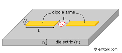
Figure 1. Model of printed dipole antenna based on differential feeding.

Layers Setup

First load up Ansoft Designer, then go to Project > Insert Planar EM Design to launch the MOM simulator. A window will appear asking you to choose a layout technology (substrate) as shown in Fig. 2. Pick MS - RT_duroid 5880 with a height of 0.010 inch. Once, you have chosen the technology, a project window will appear. Before we can setup the model, we need to remove the ground plane. To do this, go to Layout > Layouts and the Edit Layers window will appear. Select the ground layer and then click on Remove Layer. The Edit Layer window should look like Fig. 3, when the ground later is removed.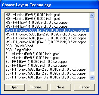

Figure 2. Choose layout technology window.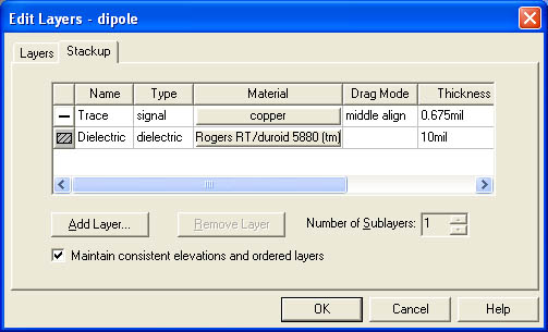

Figure 3. Layers dialog box.

Model Setup

We are now ready to start drawing the printed dipole. Before doing so, we first need to estimate what the length of the dipole should be. Since we are interested in the first resonance, a half-wavelength dipole will be designed. Therefore, the length of each arm should be around a quarter wavelength at 3.0 GHz. At 3.0 GHz, the free space wavelength is 100 mm, therefore each dipole arm will be 25 mm long. The width of the dipole arms will be set to 5 mm and the gap between the two arms will be set to 1 mm. Since, the electric field will fringe at the end of the dipole arms, the actual length of the dipole should be a little shorter than a half-wavelength. An optimization will be performed on the dipole arm length for 3.0 GHz resonance. As a result, the dipole model will be parameterized; the arm length (L), arm width (W), and the gap (g) will be set as variables.

The first dipole arm will be drawn. First select the rectangle tool and just draw a random rectangle. Next, double click on the rectangle and for Pt. A enter -g/2, -W/2 and for Pt. B enter -L/2-g/2, W/2. A dialog box asking for the value of each variable will appear, enter the following for each:

g: 1 mm
W: 5 mm
L: 50 mm

For the other dipole arm, do the same as above except change the x-coordinates of Pt. A and Pt. B to g/2 and L/2+g/2, respectively. Your completed geometry should look like Fig. 4.

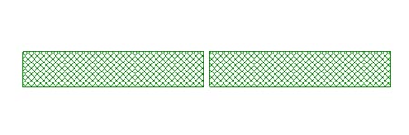
Figure 4. Dipole antenna model.

Excitation Setup

A differential excitation has to be applied in the gap separating the two dipole arms. To setup the excitation port, go to Edit > Select Edges and select the gap edge of the first drawn dipole arm as shown in Fig. 5.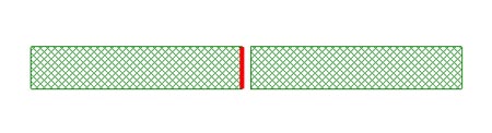

Figure 5. Selected edge for port definition.

Next, assign an edge port to the selected edge by going to Draw > Edgeport. The completed port needs a reference in order to be defined correctly since there is no ground plane. The edge of the other dipole arm will be used as the reference to create a differential port. To create the diffential port, select the other dipole arm's gap edge and go to the port definition in the project tree, right-click on the port, and then select Add Reference as shown in Fig. 6.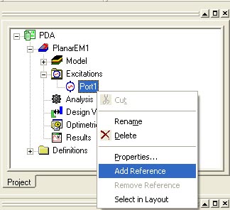

Figure 6. Differential port setup.

Analysis Setup

To setup the analysis, go to Planar EM > Solution Setup > Add Solution Setup. Since this is a geometrically simple structure, a fixed mesh will give an accurate result. Use a fixed mesh with a frequency of 4.0 GHz. In addition, add a frequency sweep from 2.0 GHz to 4.0 GHz by going to Planar EM > Solution Setup > Add Frequency Sweep; do an interpolating sweep from 2.0 GHz to 4.0 GHz with 201 points. Next, analyze the problem.

Plotting Results

After the simulation is finish, we can plot the real and imaginary parts of the input impedance over the 2.0 Ghz to 4.0 GHz range to confirm the resonant frequency. Fig. 7 shows the resulting input impedance; the results show that the dipole resonants at 2.75 GHz (Imag(Zin)=0). As a result, we need to optimize the dipole arm length to obtain resonance at 3.0 Ghz.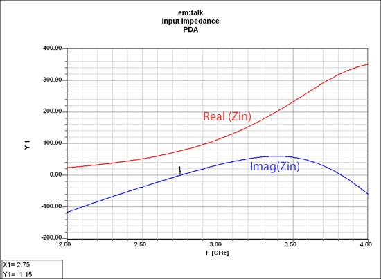

Figure 7. Input impedance of un-optimized printed dipole.

Optimization

To setup the optimization, go to Planar EM > Optimetrics Analysis > Add Optimization and a window will appear. In the optimization window, click on Add and then click on Edit Calculation. In the Edit Calculation dialog, create a new calculation called Zin_Imag and define it as im(Z(Port1,Port1)). Next, click on the Edit Calc Range and set it to a single frequency at 3.0 GHz. For the Condition set it to "=" and a Goal of 0. The completed window should look like Fig. 8.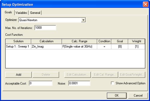

Figure 8. Optimization setup.

Next, the variable for optimization has to be setup. Click on the Variables tab of the Optimization window. Click on Advanced and setup the options to be like Fig. 9. ,/p>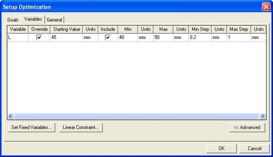

Figure 9. Variable setup.

Then, run the optimization and Ansoft Designer will automatically update the dipole length with the optimized value. The optimization determines that L should be 45.74 mm long. The resulting input impedance chart with the optimized dipole length is shown in Fig. 10; the input impedance at 3.0 Ghz is Zin = 78 Ohms. A discrete frequency sweep at 3.0 Ghz was performed and the resulting far-field pattern is shown in Fig. 11.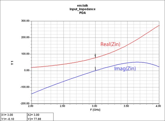

Figure 10. Input impedance with optimized dipole length.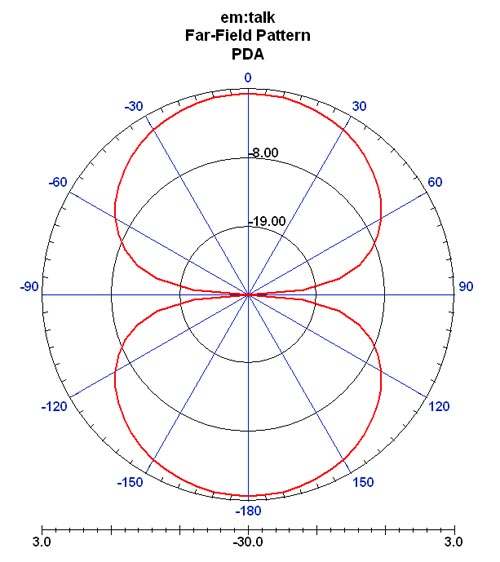

Figure 11. Far-field pattern at 3.0 GHz.