HFSS Tutorial 2

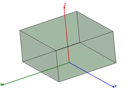
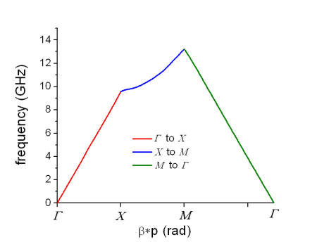
Dispersion Diagram Basics

We want to use HFSS to obtain a dispersion diagram for the first mode for a parallel plate waveguide. A dispersion diagram is a plot of propagation constant versus frequency; a dispersion diagram basically tells you how much phase shift a material has at a given frequency. Since a parallel plate waveguide allows for waves to travel in two-dimensions, its propagation constant can be written as a vector quantity, β = xk_x + yk_y. In order to generate the dispersion diagram, a unit-cell has to be defined and the appropriate periodic boundary conditions (PBCs) have to be applied. For the sake of simplicity and that a parallel plate waveguide can be treated as a periodic structure, a symmetric unit-cell (square of size p x p mm²) is defined as shown in Fig. 1.

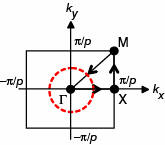
In addition, the Brillouin zone is shown with the high-symmetry points defined as

Г = (k_xp = k_yp = 0)

Х = (k_xp = π, k_yp = 0)

М = (k_xp = k_yp = π)

The Brillouin zone is the most fundamental region for defining the propagation vector for a unit-cell; basically if one can define all the propagation vectors in the Brillouin zone, one obtains the entire characteristic of the entire periodic structure. Therefore the dispersion diagram will start at Г then to Х then to M and back to Г as indicated by the path depicted on the Brillouin zone.

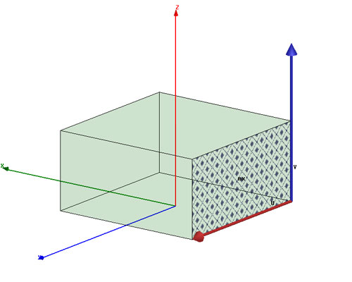
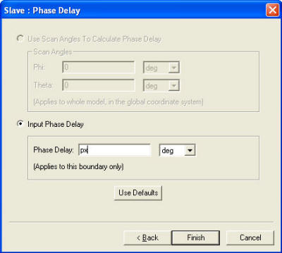
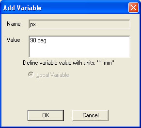
Model Setup

First we must configure HFSS to use its eigenmode solver; HFSS>Solution Type...>Eigenmode. Next, the unit-cell of parallel plate waveguide has to be drawn in HFSS. It consists of rectangular substrate as shown in Fig. 1. The dimensions of the unit-cell are 5.0x5.0x2.54 mm³ and the substrate material is Rogers RT/duroid 6010/6010LM.

Periodic Boundary Conditions

1. Select the negative y-z face of the unit-cell and assign a Master Boundary Condition (mx); you have to define the U Vector which starts at (-2.5, -2.5, 0) and ends at (-2.5, 2.5,0). The completed boundary assignment should look like Fig. 3. Next select the positive y-z face of the unit-cell and assign a Slave Boundary Condition (sx). Again define the U Vector which starts at (2.5, -2.5, 0) and ends at (2.5, 2.5, 0). Then input the phase delay using a variable (px) as shown in Fig. 4 and input an initial value (90 deg) as shown in Fig. 5. *Do not forget to put in “deg.”

2. Do the same to the x-z faces of the unit-cell. Label the master as my and the slave as sy. For sy make sure to reverse the V Vector and use a variable (py) and input an initial value (0 deg). *Do not forget to put in “deg.”

Analysis/Optometrics Setup

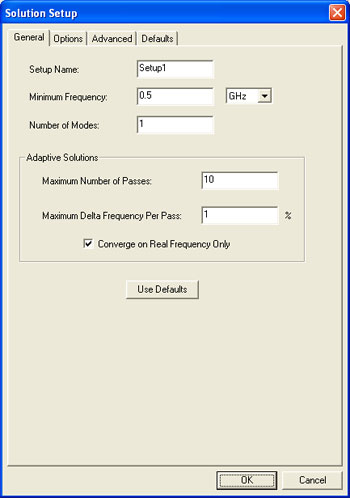
Before the eigenmode analysis can be started, several steps need to be completed first. First, add a solution setup and input the values as depicted in Fig. 6. In addition, in the options tab of the Solutions Setup, input a minimum converged passes of 3.
 

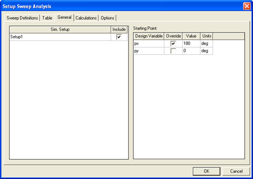
Next, parametric sweeps need to be added. So chose HFSS>Optometrics Analysis>Add Parametric. You will need to do this three times for each of the high-symmetry points of the Brillouin zone.

For the first parametric sweep, we will go from Г to Х and this will be labeled 1_Gamma2X. Add a linear step sweep for the variable px from 15 deg to 180 deg with 15 deg steps. In the Options tab make sure to check both Save Fields and Mesh and Copy geometrically equivalent meshes.

For the second parametric sweep, we will go from Х to M and this will be labeled 2_X2M. Add a linear step sweep for the variable py from 15 deg to 180 deg with 15 deg steps. We have to set px to 180 deg. To do this go to General tab and check override for px and input 180 deg as shown in Fig. 7.  In the options tab make sure to check both Save Fields and Mesh and Copy geometrically equivalent meshes.

For the third parametric sweep, we will go from M to Г and this will be labeled 3_M2Gamma. Add a linear step sweep for the variable px from 15 deg to 180 deg with 15 deg steps and also for the variable py. Select both of these sweeps and Sync them as shown in Fig. 8. In the options tab make sure to check both Save Fields and Mesh and Copy geometrically equivalent meshes.

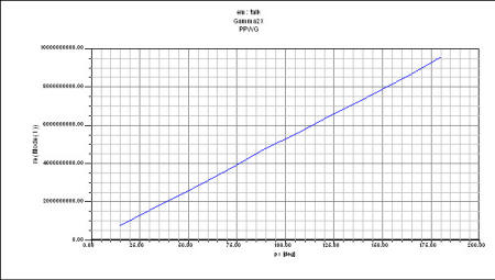
Plotting Results

Plots for each parametric sweep have to be made. For the Г to Х parametric sweep, create a report and use the default values (Eigenmode Parameters, Rectangular Plot). In the Sweep tab, choose Sweep Design and Project variable values and choose px values from 15 deg to 180 deg and for py select only 0 deg. For the Y tab, choose Eigen Modes>Mode(1)>re. We only wish to look at the real part of the eigenmode, the imaginary part is due to loss which is ignored since a parallel plate waveguide’s loss is negligible for the fundamental mode. The finished plot should look like Fig. 9.

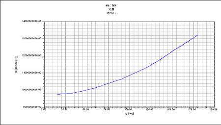
To plot the X to M parametric sweep, do the same as for the Г to Х parametric sweep report. However, make py as the primary sweep and set px to 180 deg. The finished plot should look like Fig. 10.

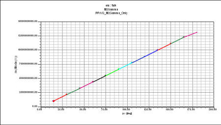
To plot the M to Г parametric sweep, do the same as for the previous plots, but this time select values of 15 deg to 180 deg for both px and py. However, the resulting plot will just be a series of unconnected dots. This is because HFSS’s plotting function does not know which order to connect them. You can easy export the data and plot it yourself or create another HFSS design and only add an M to Г parametric sweep. HFSS will then connect the dots in the results as shown in Fig. 11. The complete dispersion diagram is shown in Fig. 12; it was plotted by exporting the eigenvalues obtained from HFSS and using an external plotting program.

Discuss this in the forums.