HFSS Tutorial 4

Left-Handed Materials: Effective Medium Approach

Materials with simultaneous negative permittivity and permeability referred to as left-handed materials was first theorized in the 1960s. Left-handed materials support backward-waves (i.e. phase and group velocity are opposite) and therefore have a negative refractive index. In this tutorial, the negative refractive index of a left-handed material is used to demonstrate a flat lens. This concept is based on Snell's Law of Refraction and is depicted in Fig. 1. If a point source is placed in the right-handed medium (RHM), a image of the point source will be reproduced in the left-haned medium (LHM). The left-handed medium for the flat lens is realized in HFSS with an effective medium approach; the substrate is assigned a constant negative value of permittivity and permeability.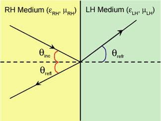

Figure 1. Snell's law applied to the interface of a RHM/LHM.

Left-handed materials have lead to novel microwave antennas, resonators, waveguides, and lenses. In this tutorial, a novel flat lens is demonstrated using an effective medium approach. Such a flat lens is not possible with conventional microwave substrates or materials. The following topics are covered:

Model Setup
Effective Medium Approach
Voltage Source Setup
Analysis Setup
Plotting Field Results

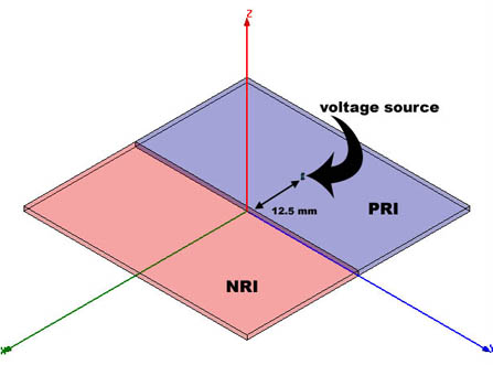
Model Setup

To realize the lens, a parallel plate waveguide is half-filled with a RHM and half-filled with a LHM. The refractive index of the LHM will be the negative of the RHM. A point source is placed in the RHM and it is expected that its image will occur in the LHM. Fig. 2 shows the model setup used for the simulation. The size of each region is 25.0x20.0x1.0 mm³ and radiation boundary is placed on all 4 edges of the parallel plate waveguide. The entire parallel plate is realized by two separate rectangular parallel plates. A voltage point source is placed in the RHM 12.5 mm away from the RHM/LHM interface.

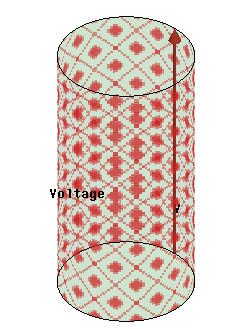
Figure 2. Model of flat lens structure used for simulation.

Effective Medium Setup

In this section, the RHM and LHM's permittivity and permeability is setup in HFSS. The RHM will have a positive refractive index (PRI) of n=3.16, while the LHM will have a negative refractive index (NRI) of n=-3.16, where n=sqrt(μ·ε). To setup the permittivity and permeability required to realize each region, a RHM and a LHM needs to be created. To do this, select the RH region of the parallel plate waveguide and then Assign Material. Once in the Assign Material window, choose View/Edit Material and create a new material named RH_Material with a permittivity of 10.0 and a permeability of 1.0. Do the same for the LH region of the parallel plate waveguide, but this time make a new material named LH_Material with a permittivity of -11.1 and permeability of -0.9. The difference in the numerical values between the RHM and LHM is to create a impedance mismatch to prevent the formation of constructive interference at the interface.

Voltage Source Setup

A voltage source (cylindrical waves) is placed 12.5 mm away from the interface in the RHM. To do this, a cylinder with a height of 1.00 mm and a radius of 0.25 mm is created and assigned the RH_Material. To setup the excitation select the face of the cylinder and go to Assign Excitation>Voltage... leave the default values but for the E-Field Direction, setup a New Line... from the bottom of the cylinder to the top. Fig. 3 shows the completed voltage source with the line direction.

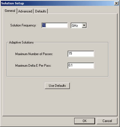
Figure 3. Close-up of voltage source (similar to coaxial probe).

Analysis Setup

To simulate the flat lens, an analysis setup has to be performed. The solution frequency used is 10.0 GHz with an adaptive pass of 15 and a Delta of 0.1. Fig. 4 shows the Analysis Setup window with the relevant values.

Figure 4. Analysis setup window.

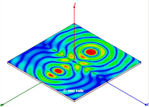
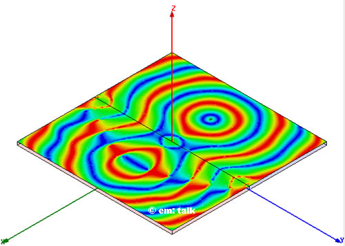
Plotting Field Results

After the analysis is completed, the top of the parallel plate is selected and the electric field is plotted. Fig. 5 shows the electric field magnitude, while Fig. 6 shows the electric field phase.

Both figures confirm that the flat lens works. In addition, Fig. 7 shows the animated electric field magnitude as a function of phase. Since the LHM supports a backward-wave, the field in the LH region appears to be moving backwards.

Figure 5. Electric field magnitude plot.

Figure 6. Electric field phase plot.

Figure 7. Animated electric field magnitude plot.